
Featured Post

Excel SUMIF Function Explained with Real Examples

If you work with numbers in Excel, there's one function you must master: SUMIF. It’s simple, powerful, and one of the most searched formulas globally. Whether you’re managing sales data, budgets, or reports, SUMIF helps you add values based on conditions — no filters needed. WHAT IS THE SUMIF FUNCTION? The SUMIF function adds numbers in a range only if they meet a given condition. Syntax: =SUMIF(range, criteria, [sum_range]) - range – The cells to test against your condition- criteria – The condition to match - sum_range (optional) – The cells to actually sum (if different from range) Example 1: Add Sales Greater Than 100 Example Data: Product Sales A 120 B 80 C 150 If you need the sum of product whose sales more than 100 then the formula will be: =SUMIF(A2:B4,">100") Result: 270 (120 + 150) Example 2: Sum Based on Text Match Example Data: Product Sales ...

How to Remove Virus from Removable Disk

Introduction

Are you wondering how to remove a virus from a removable disk like a USB drive, external hard drive, or SD card? Removable disks can easily become infected with viruses that corrupt files, create shortcuts, or hide valuable data. In this SEO-optimized guide, we’ll show you how to remove viruses from your removable disk in simple steps, helping you keep your files safe, and your devices secure.

Why Do Removable Disks Get Viruses?

Viruses spread to removable disks when they’re connected to infected computers or used in public or shared computers. Understanding how viruses spread and how they affect your removable disk is essential for keeping your data safe. This guide will cover the most common signs of a virus on a USB drive and step-by-step instructions to remove viruses from removable disks.

Signs Your Removable Disk May Be Infected with a Virus

Before you start virus removal, here are some common signs your removable disk is infected:

  1. Unusual Files – New, strange files or folders appear, often with .exe, .vbs, or .scr extensions.
  2. Missing or Hidden Files – Files disappear or turn into shortcuts, preventing easy access.
  3. Slow or Strange Behaviour – The disk responds slowly, or unusual behaviour occurs when connected.

These signs indicate you need to learn how to remove viruses from your removable disk quickly to avoid further harm.

Step 1: Disable Autorun on Windows to Prevent Virus Spread

Disabling Autorun on Windows is a preventive step that can stop viruses on USB drives and SD cards from automatically running.

  1. Go to the Start Menu and search “gpedit.msc” to open Local Group Policy Editor.
  2. Navigate to Computer Configuration > Administrative Templates > Windows Components > AutoPlay Policies.
  3. Double-click Turn off AutoPlay and set it to Enabled.
  4. Restart your computer to apply the change.

Disabling Autorun can be an effective first step to prevent virus infections on removable disks.

Step 2: Scan Your Removable Disk with Trusted Antivirus Software

Running an antivirus scan is one of the most effective methods to remove viruses from removable disks.

  1. Insert your removable disk into the USB port.
  2. Open your antivirus software (e.g., Windows Defender, Avast, Norton, etc.).
  3. Choose Scan External Devices and select your removable disk.
  4. Delete or quarantine any threats found during the scan.

Keeping your antivirus software updated ensures you’re protected from the latest virus strains that might target your removable disks.

Step 3: Use Command Prompt to Unhide Files and Remove Virus Shortcuts

If your files have turned into shortcuts or are hidden, Command Prompt can help you restore them.

  1. Press Win + R, type cmd, and press Shift + Enter to open the Command Prompt window in Administrator mode.
  2. Type this command:

attrib -h -r -s /s /d X:\*.*

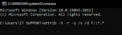
Replace X with the letter assigned to your removable disk.

  1. Press Enter to execute the command, which will unhide your files and remove any shortcuts created by viruses.

Using Command Prompt is a powerful and effective way to recover files and clean your disk from viruses.

Step 4: Manually Delete Suspicious Files

After unhiding files with Command Prompt, open File Explorer and manually look for strange files on your removable disk. Any unfamiliar files with suspicious extensions, such as .exe, .vbs, or .scr, may be viruses. Delete suspicious files carefully, but ensure they’re not legitimate files required by the disk.

Step 5: Format the Removable Disk if Necessary

If virus removal steps haven’t worked, you may need to format the removable disk to delete all files, including any viruses. Formatting your removable disk should be your last resort, as it erases all data.

  1. Open File Explorer, right-click on your removable disk, and select Format.
  2. Choose the File System (NTFS or FAT32) and click Start.
  3. Wait until the formatting process completes, then recheck your disk.

Formatting will remove all viruses but will also delete all your data, so back up any important files before formatting.

Preventive Tips to Keep Removable Disks Virus-Free

  1. Regular Scanning – Run antivirus scans on all external disks regularly to detect threats early.
  2. Avoid Public Computers – Limit use on public or shared computers, which often carry a higher risk of viruses.
  3. Update Antivirus Software – Always keep your antivirus software updated to protect from new viruses.
  4. Enable Write Protection – Use write protection on important files when they don’t need to be edited to prevent modifications by viruses.

Conclusion

Following these steps will help you remove viruses from your removable disk and protect your USB drives, SD cards, and other removable storage devices. Whether using antivirus software, Command Prompt, or preventive measures, it’s possible to keep your removable disks virus-free and protect your data. Remember to regularly back up important files and scan all external storage devices before connecting them to your computer.

By staying vigilant and using these virus removal methods, you’ll ensure your removable disks stay secure and free from malware.


Comments

Popular

FILTER Function in Excel with Example

Excel is a powerful tool with a myriad of functions that can simplify data management and analysis. Among its extensive repertoire, the FILTER function stands out for its ability to dynamically extract data based on specific criteria. While it may not be as widely known as functions like VLOOKUP or SUMIF, FILTER can be a game-changer when it comes to handling complex data sets.  In this blog post, we’ll dive deep into the FILTER function, exploring its syntax, use cases, and practical examples. By the end, you’ll be able to harness this function to make your data analysis more efficient and dynamic. What is the FILTER Function? The FILTER function is a part of Excel’s suite of dynamic array functions, introduced in Excel 365 and Excel 2019. It allows you to extract a range of data that meets specific criteria, automatically adjusting as the data changes. This makes it a powerful tool for creating custom views of your data without the need for complex formulas or manual adjustm...

IFERROR Function in Excel with Example

  When working with large datasets in Excel, errors are inevitable. Whether it's a division by zero, missing values, or formula mistakes, errors can disrupt your calculations and analysis. The Excel IFERROR function is your go-to tool to handle these issues effectively. In this guide, we’ll cover how to use IFERROR, its syntax, practical use cases, and why it’s essential for error-proofing your Excel work. What is the IFERROR Function? The IFERROR function in Excel is designed to catch errors in formulas and replace them with a value of your choice. Instead of leaving error messages like #DIV/0!, #N/A, or #VALUE! in your spreadsheet, you can display something more useful—like a zero, blank cell, or custom message. This function is particularly useful when you’re dealing with complex formulas or pulling data from external sources that may have missing or incorrect values. Syntax of the IFERROR Function =IFERROR(value, value_if_error) value : The expression or form...

SWITCH Function in Excel with Example

In the world of Excel formulas, versatility and efficiency are key. One such tool that enhances both is the SWITCH function, which allows you to test an expression against multiple conditions and return the corresponding result. This function is often used in place of multiple IF statements, making your formulas more readable and easier to manage. What is the SWITCH Function? The SWITCH function in Excel evaluates an expression against a list of possible values and returns a corresponding result based on the first matching value. If no match is found, it can return a default result. This function is particularly useful for simplifying complex IF statements that involve several comparisons. Syntax of SWITCH Function The syntax for the SWITCH function is as follows: =SWITCH(expression, value1, result1, [value2, result2], ..., [default]) Expression : The value or cell that you want to evaluate. Value1, Value2, ... : The values you want to compare against the e...

HLOOKUP Function in Excel with Example

If you've ever worked with horizontal datasets in Excel and needed to find a specific value, the HLOOKUP function is your go-to tool. Short for "Horizontal Lookup," HLOOKUP allows you to search for a value across the top row of a table and return information from a specified row below. It’s particularly useful when managing spreadsheets with data organized in a horizontal format. In this post, we'll dive into how HLOOKUP works, why it’s useful, and how to apply it in various scenarios. What is HLOOKUP? The HLOOKUP function searches for a specific value in the top row of a table and returns data from a row you specify. It’s like the vertical counterpart, VLOOKUP, but designed for datasets where values are arranged horizontally. HLOOKUP Syntax: =HLOOKUP(lookup_value, table_array, row_index_num, [range_lookup]) lookup_value : The value you want to find in the first row. table_array : The range of data you want to search in. row_index_num : The ...

IFS Function in Excel with Example

In the world of Excel, performing logical tests is an essential skill that helps users analyse data, make decisions, and solve problems efficiently. One of the most powerful functions in Excel for this purpose is the IFS function. While many are familiar with the basic IF function, the IFS function takes conditional testing to the next level by allowing you to test multiple conditions at once, without needing to nest multiple IF statements. In this post, we will explain the working of the Excel IFS function, its usage, advantages, and provide practical examples to showcase how this function can simplify your workflow. What is the IFS Function? The IFS function in Excel is a logical function introduced in Excel 2016 that simplifies complex conditional tests. It evaluates multiple conditions in the order specified and returns a value corresponding to the first TRUE condition. If none of the conditions are met, an error will be returned unless a default condition is provided. The ...

IF function in excel with Example

The Excel IF formula is one of the most frequently used functions in spreadsheet operations. Its power lies in its ability to create logical comparisons between a value and what you expect. The function allows Excel users to automate tasks, analyse data more efficiently, and manage large datasets without manually reviewing every entry. In this detailed guide, you’ll learn how to harness the full potential of the IF formula, and we’ll dive deep into its variations and best practices. What is the IF Formula? At its core, the Excel IF formula performs a logical test, and based on the outcome of that test, it returns one of two results. It’s a basic yet versatile function that can handle a wide range of applications in financial modelling, data analysis, inventory management, and even project planning. Here’s the syntax for the IF formula: =IF(logical_test, value_if_true, value_if_false) In this syntax: 1.   logical_test : This is the condition or criteria that you want to ...

Excel SUMIF Function Explained with Real Examples

If you work with numbers in Excel, there's one function you must master: SUMIF. It’s simple, powerful, and one of the most searched formulas globally. Whether you’re managing sales data, budgets, or reports, SUMIF helps you add values based on conditions — no filters needed. WHAT IS THE SUMIF FUNCTION? The SUMIF function adds numbers in a range only if they meet a given condition. Syntax: =SUMIF(range, criteria, [sum_range]) - range – The cells to test against your condition- criteria – The condition to match - sum_range (optional) – The cells to actually sum (if different from range) Example 1: Add Sales Greater Than 100 Example Data: Product Sales A 120 B 80 C 150 If you need the sum of product whose sales more than 100 then the formula will be: =SUMIF(A2:B4,">100") Result: 270 (120 + 150) Example 2: Sum Based on Text Match Example Data: Product Sales ...

VLOOKUP Formula in Excel with Example

VLOOKUP (Vertical Lookup) is one of Excel’s most powerful and widely used functions. It allows users to search for a value in the first column of a range and return a corresponding value in the same row from another column. Whether you are managing inventory, financial data, or customer information, VLOOKUP helps save time by automating data retrieval across large datasets. How VLOOKUP Works VLOOKUP scans the column of a given range for a specific value, then returns the corresponding data from a different column. Here’s the basic structure of the VLOOKUP formula: =VLOOKUP(lookup_value, table_array, col_index_num, [range_lookup]) lookup_value : The value you want to find in the first column of the table. table_array : The range that contains the data (columns from which the function will pull). col_index_num : The column number from which you want to retrieve the value. [range_lookup] : Optional parameter (TRUE for approximate matches, FALSE for ex...